Extracting value from OSINT: Estimating carbon credits in Paraguay
Disclaimer that this topic is quite niche and only scratches the surface of what was done in the process. Let me know if you are interested in a long read to get more insights!
Introduction
Open Source Intelligence (OSINT) is a source for instant, cheap, and maintained datasets on various topics. Most OSINT datasets cover social-economic matters, yet over the years more and more geographical, geological, and climate-related datasets have been aggregated by research teams.
For one of the project I did in the past, Aboveground/Belowground Biomass (AGB/BGB) was the main metric of interest to gauge the potential to extract the power to absorb tCO2eq, mainly how much carbon dioxide can be taken out through the biodiversity. AGB is the estimation of living biomass (seeds, branches but also animals) where BGB is only on estimate on top of AGB, which revolves mostly around 10%.
One specific dataset, the ESA Climte Change ABG estimate of 2021, covers the need to assess the aforementioned values for dedicated areas. Especially for vast areas, which not only host forests but also savannahs, shrubs, and water, the dataset provides a good estimate. Nevertheless, one of the key limits is the large deviation in estimates and are flagged by the authors/creators of the dataset by providing standard deviations. This is due to the methodology of the authors, mainly relying on infrared bursts and their reflection to calculate the AGB/BGB density. Especially for high-density regions (>200 t/cubicmetre), the offset can grow to as much as 35%.
To not solely rely on the values and the standard deviations of this set, I found an additional solution to limit the error of the assessment to 20% compared to any on-site assessment of the territory, which is the Dynamic World dataset provided by Google. You will see how these two will be merged later on.
Most of these tasks take an analyst week(s) of work through chats with locals, experts & additional analysis to come to a conclusion, where the workload increases likely linearly with the size of a lot. We therefore want to focus on available data to get as close as possible to actual values & validate how close we come to the actual results.
Matching the right parts with known types
The first task is to identify the right parts within a region of interest to attribute them to the right AGB/BGB value afterwards. Especially the split between is necessary to identify potential spaces of growth and ongoing plantations. A forest will have a higher chance of high AGB than a lake for example. To bring more clarity to what these parts are, relevant regions mainly consist of “forest”, “savannah” & “water”, with “wetlands” being much rarer in regions.
This information is tough to extract from the original dataset, as the contrast between the different parts can be obvious (savannah and water will have less AGB than a forest) but not granular enough to differentiate between low AGB parts (mainly savannah/water). Even though those can be identified with manual analysis, we want to avoid any side-step away from automation.
For this step, we might work with the deforestation map provided by JAXA, dating back to 2020, to identify potential differences between the result of the initial categorization and the newly provided one. The deforestation map specifically focuses on whether or not a 30x30m square is mainly populated by trees, water or anything else. This classifying approach helps to easily fit the relevant information into the aforementioned categories. Yet an additional drawback is the timeframe taken into account: 2018 is not recent enough to cover all changes, leading to being not as accurate as one might think.
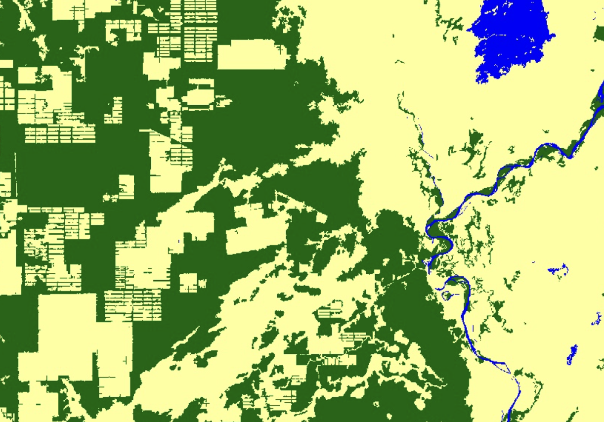
JAXA & their deforestation map replotted
We, therefore, rely on the last resource available, the Dynamic World dataset provided by Google. For every 100x100m square, an algorithm determines what category fits the best in terms of the environment. Note that this is constantly (as clouds can conver some surface) updated and based on a trained network with a very specific training processes. Some classes taken into account have been highlighted above, the rest can be looked up here.
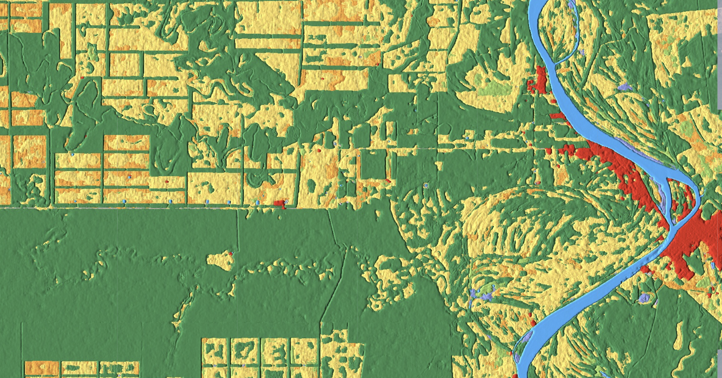
Dynamic World is such as exciting project
Based on the categories, we aggregate the most convienent together or leave them out as they might not be as relevant. Wetlands and water can be aggregated, and so do grass, shrub/scrub & bare categories. Recent, additional research brought up further datasets, yet felt too experiemental at this early stage. One option could be to use soil data to roughly estimate AGB/BGB directly and associate it to either group. More advanced monitoring and modelling would include regional aspects being taken into account within the next step.
At this stage, we have segmented squares for our region of interest, but we yet have to aggregate these with their respective AGB values and determine how large the potential in the respective region.
Getting the best estimates for AGB/BGB for each segment
With all the different parts defined for the region of interest, we can move on to identify what the AGB/BGB estimate for each square is. Note that in the prior step, we get the label of each 10x10 m block to define the limits of each part to assess and check what squares should be taken into account for the AGB calculation rather than including waters & wasteland in the comparison.
We can download these limits and the Dynamic World dataset locally to have a look in QGIS (your favourite GIS software) after having calculated anyting prior on the online version of the firstly mentioned dataset within Earth Engine (highighted above). This is then mapped to the ESA dataset by leveraging in Pyton & overlayed to compare the regions of interest with their respective AGB & BGB estimates. One key observation during the validation process was an underestimate of all AGB/BGB for all parts compared to the actuals. Large discrepancies were observable even when accounting for the standard deviation (± 35%), which resides in a separate dataset.
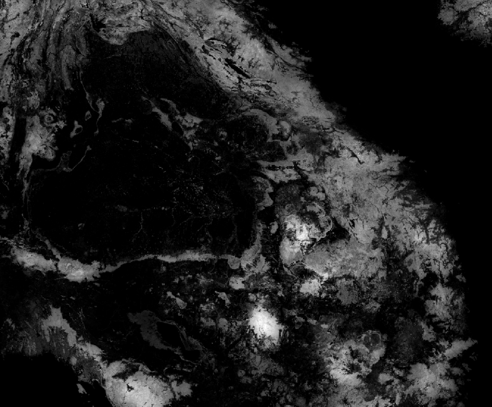
Happy I do not have to open QGIS everytime to calculate the AGB of squares! (Dark means high AGB)
As a solution, I introduce a longer-ranging region to get a better estimate of the actual values for the respective sub-region such as forest, wasteland and water. For most regions, we draw a disk of double the size to encompass all parts appearing in the region to the same share. Whilst calculating their AGB/BGB share for the new region, we take the standard deviation/uncertainty into account, as we account for the largest possible margin for each part. We take the median as the final result for each part as the new AGB/BGB estimate into account.
Over the REDD projects analysed, the additional markup between initial AGB/BGB and calculated results is +10-20% for each subclass. Class-specific behaviour can be observed, where forests mainly take a +20% bump, compared to low AGB/BGB parts which float around ±10%. When comparing the new calculated AGB/BGB values and converting them into tC02e, a consistent 20% offset between the on-ground valuation and the calculated estimates throughout all classes. Since a 20% discount can be priced in and the tendency is always undervalued, the current method is established as a standard.
Conclusion
Estimates of AGB/BGB values of forests remain a tidious task in the current days, especially if you are not present. Having a true value-add from afar and driving the adoption of data-driven tooling in the sector is amazing, although other amazing venture out there do a better job than this (hi Ororatech!). Nevertheless, I hope that this somewhat highlights the value of OSINT in one specific way and shows that there is already a plethora of data out there ready to be used.